Applets:Bessel Functions of the First Kind: Unterschied zwischen den Versionen
Tasnad (Diskussion | Beiträge) |
|||
| Zeile 1: | Zeile 1: | ||
| − | {{LntAppletLinkEn| | + | {{LntAppletLinkEn|besselFuns_en}} |
==Applet Description== | ==Applet Description== | ||
| Zeile 185: | Zeile 185: | ||
==Once again: Open Applet in new Tab== | ==Once again: Open Applet in new Tab== | ||
| − | {{LntAppletLinkEn| | + | {{LntAppletLinkEn|besselFuns_en}} |
Version vom 9. Juni 2020, 21:46 Uhr
Inhaltsverzeichnis
Applet Description
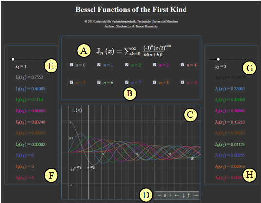
This applet allows the calculation and graphical representation of the Bessel functions of the first kind and $n$–th order according to the series representation:
- $${\rm J}_n (x) = \sum\limits_{k=0}^{\infty}\frac{(-1)^k \cdot (x/2)^{n \hspace{0.05cm} + \hspace{0.05cm} 2 \hspace{0.05cm}\cdot \hspace{0.05cm}k}}{k! \cdot (n+k)!} \hspace{0.05cm}.$$
- The functions ${\rm J}_n (x)$ can be represented graphically for the order $n=0$ to $n=9$ in different colors.
- The left output provides the function values ${\rm J}_0 (x = x_1)$, ... , ${\rm J}_9 (x = x_1)$ for a slider-settable value $x_1$ in the range $0 \le x_1 \le 15$ with increment $0.5$.
- The right output provides the function values ${\rm J}_0 (x = x_2)$, ... , ${\rm J}_9 (x = x_2)$ for a slider-settable value $x_2$ (same range and value increment like on the left).
Theoretical Background
General Information about the Bessel Functions
Bessel functions (or cylinder functions) are solutions of the Bessel differential equation of the form
- $$x^2 \cdot \frac{ {\rm d}^2}{{\rm d}x^2}\ {\rm J}_n (x) \ + \ x \cdot \frac{ {\rm d}}{{\rm d}x}\ {\rm J}_n (x) \ + \ (x^2 - n^2) \cdot {\rm J}_n (x)= 0. $$
This is an ordinary second-order linear differential equation. The parameter $ n $ is usually integer, also in this program. These mathematical functions, introduced by Friedrich Wilhelm Bessel in 1844, can also be represented in closed form as integrals:
- $${\rm J}_n (x) = \frac{1}{2\pi}\cdot \int_{-\pi}^{+\pi} {{\rm e}^{\hspace{0.05cm}{\rm j}\hspace{0.05cm}\cdot \hspace{0.05cm}[\hspace{0.05cm}x \hspace{0.05cm}\cdot \hspace{0.05cm}\sin(\alpha) -\hspace{0.05cm} n \hspace{0.05cm}\cdot \hspace{0.05cm}\alpha \hspace{0.05cm}]}}\hspace{0.1cm}{\rm d}\alpha \hspace{0.05cm}.$$
The functions ${\rm J}_n (x)$ belong to the class of Bessel functions of the first kind (German: Besselfunktionen erster Art). The parameter $n$ is called the Order.
Annotation: There are a number of modifications of the Bessel functions, including the Bessel functions of the second kind named ${\rm Y}_n (x)$. For integer $n$, ${\rm Y}_n (x)$ can be replaced by ${\rm J}_n (x)$ functions. However, in this applet, only the first kind Bessel functions ${\rm J}_n (x)$ are considered.
Properties of the Bessel Functions
$\text{Property (A):}$ If the function values for $n = 0$ and $n = 1$ are known, then the Bessel function for $n ≥ 2$ can be determined iteratively:
- $${\rm J}_n (x) ={2 \cdot (n-1)}/{x} \cdot {\rm J}_{n-1} (x) - {\rm J}_{n-2} (x) \hspace{0.05cm}.$$
$\text{Example (A):}$ Let ${\rm J}_0 (x = 2) = 0.22389$ and ${\rm J}_1 (x= 2) = 0.57672$. From this it can be calculated iteratively:
- $${\rm J}_2 (x= 2) ={2 \cdot 1}/{2} \cdot {\rm J}_{1} (x= 2) - {\rm J}_{0} (x= 2) = 0.57672 - 0.22389 = \hspace{0.15cm}\underline{0.35283}\hspace{0.05cm},$$
- $${\rm J}_3 (x= 2) ={2 \cdot 2}/{2} \cdot {\rm J}_{2} (x= 2) - {\rm J}_{1} (x= 2) = 2 \cdot 0.35283 - 0.57672 = \hspace{0.15cm}\underline{0.12894}\hspace{0.05cm},$$
- $${\rm J}_4 (x= 2) ={2 \cdot 3}/{2} \cdot {\rm J}_{3} (x= 2) - {\rm J}_{2} (x= 2) = 3 \cdot 0.12894 - 0.35283 = \hspace{0.15cm}\underline{0.03400}\hspace{0.05cm}.$$
$\text{Property (B):}$ The symmetry relationship applies ${\rm J}_{–n}(x) = (–1)^n · {\rm J}_n(x)$:
- $${\rm J}_{-1}(x) = - {\rm J}_{1}(x), \hspace{0.3cm}{\rm J}_{-2}(x) = {\rm J}_{2}(x), \hspace{0.3cm}{\rm J}_{-3}(x) = - {\rm J}_{3}(x).$$
$\text{Example (B):}$ For the spectrum of the analytic signal, the following applies to Phase Modulation of a sinusoidal signal:
- $$S_{\rm +}(f) = A_{\rm T} \cdot \sum_{n = - \infty}^{+\infty}{\rm J}_n (\eta) \cdot \delta \big[f - (f_{\rm T}+ n \cdot f_{\rm N})\big]\hspace{0.05cm}.$$
Denote this
- $f_{\rm T}$ the carrier frequency (German: $\rm T$rägerfrequenz),
- $f_{\rm N}$ the frequency of the source signal (German: $\rm N$achrichtenfrequenz),
- $A_{\rm T}$ the carrier amplitude (German: $\rm T$rägeramplitude).
The parameter of the Bessel functions in this application is the modulation index $\eta$.
Based on the graphic, the following statements are possible:
- $S_+(f)$ consists here of an infinite number of discrete lines at a distance of $f_{\rm N}$.
- Thus the sectrum is in principle infinitely extended.
- The weights of the spectral lines at $f_{\rm T} + n · f_{\rm N}$ ($n$ integer) are determined by the modulation index $η$ over the Bessel functions ${\rm J}_n(η)$.
- The spectral lines are real in the case of a sinusoidal source signal and a cosinusoidal carrier and symmetrical about $f_{\rm T}$ for even $n$.
- In the case of odd $n$, a change of sign corresponding to $\text{Property (B)}$ must be taken into account.
- The Phase Modulation of another phase oscillation of source and / or carrier signal provides the same magnitude spectrum.
Applications of the Bessel Functions
The applications of the Bessel functions in nature and engineering are diverse and play an important role in physics, for example:
- Electromagnetic waves in a cylindrical waveguide,
- Solutions to the radial Schrödinger equation,
- Pressure amplitudes of inviscid rotational flows,
- Heat conduction in a cylindrical object,
- Diffusion problems on a lattice,
- Dynamics of floating bodies,
- Frequency-dependent friction in circular pipelines
- Angular resolution.
The Bessel functions are counted among the special functions because of their many applications in mathematical physics.
In the following, we restrict ourselves to a few areas that are addressed in our tutorial $\rm LNTwww$.
$\text{Example (C):} \hspace{0.5cm} \text{Use in Spectral Analysis} \ \Rightarrow \ \text{Kaiser-Bessel filter}$
The spectral leakage effect is the falsification of the spectrum of a periodic and thereby time unlimited signal due to the implicit time limitation of the discrete Fourier transform (DFT). This will be done, for example, by a spectrum analyzer
- in the time signal not existing frequency components simulated, and/or
- actually existing spectral components are obscured by sidelobes.
The task of the spectral analysis is to limit the influence of the spectral leakage effect by providing suitable window functions.
Such a window function provides, for example, the Kaiser–Bessel window ⇒ see section Special Window Functions. Its time-discrete window function with the Bessel function zero order ⇒ ${\rm J}_0(x)$, the parameter $\alpha=3.5$ and the window length $N$:
- $$w_\nu = \frac{ {\rm J}_0\big(\pi \cdot \alpha \cdot \sqrt{1 - (2\nu/N)^2}\big)}{ {\rm J}_0\big(\pi \cdot \alpha \big)}.$$
On the page Quality Criteria of Window Functions and other the parameters of the Kaiser-Bessel window are given:
- Conveniently, the large are „minimum distance between the main lobe and side lobes” and the desired small „maximum scaling error”.
- Due to the very large „equivalent noise width” the Kaiser-Bessel window cuts in the most important comparison criterion „maximum process loss” but worse than the established Hamming and Hanning windows.
$\text{Example (D):} \hspace{0.5cm} \text{Rice-Fading Channel Model}$
The Rayleigh - Distribution describes the mobile channel on the assumption that there is no direct path and thus the multiplicative factor $z(t) = x(t) + {\rm j} \cdot y(t)$ is composed solely of diffusely scattered components.
In the case of a direct component (English: Line of Sight, LoS) in the model for the mean-free Gaussian processes $x(t)$ and $y(t)$ one has to add equal components $x_0$ and/or $y_0$ :
$$\hspace{0.2cm}x(t) \hspace{0.1cm} \Rightarrow \hspace{0.1cm} x(t) +x_0 \hspace{0.05cm}, \hspace{0.2cm} y(t) \hspace{0.1cm} \Rightarrow \hspace{0.1cm} y(t) +y_0\hspace{0.05cm},$$
$$\hspace{0.2cm}z(t) = x(t) + {\rm j} \cdot y(t) \hspace{0.1cm} \Rightarrow \hspace{0.1cm} z(t) +z_0 \hspace{0.05cm},\hspace{0.2cm} z_0 = x_0 + {\rm j} \cdot y_0\hspace{0.05cm}.$$
The graph shows the Rice–Fading channel model. It can be summarized as follows:
- The real part $x(t)$ is Gaussianized with mean $x_0$ and variance $\sigma ^2$.
- The imaginary part $y(t)$ is also Gaussian (mean $y_0$, equal variance $\sigma ^2$) and independent of $x(t)$.
- For $z_0 \ne 0$, the amount $\vert z(t)\vert$ rice is distributed, from which the term „Rice–Fading” arises.
- To simplify the notation, we set $\vert z(t)\vert = a(t)$. For $a < 0$ , the amounts - WDF are $f_a(a) \equiv 0$, for $a \ge 0$ the following equation holds, where ${\rm I_0}(x)$ is the modified Besselfunktion zeroth order denotes:
- $$f_a(a) = \frac{a}{\sigma^2} \cdot {\rm e}^{ - (a^2 + \vert z_0 \vert ^2)/(2\sigma^2)} \cdot {\rm I}_0 \left [ \frac{a \cdot \vert z_0 \vert}{\sigma^2} \right ] \hspace{0.5cm}\text{with}\hspace{0.5cm}{\rm I }_0 (u) = {\rm J }_0 ({\rm j} \cdot u) = \sum_{k = 0}^{\infty} \frac{ (u/2)^{2k} }{k! \cdot \Gamma (k+1)} \hspace{0.05cm}.$$
- Between the modified Bessel function and the traditional Bessel function ${\rm I_0}(x)$ – in each case of first kind – So the connection exists ${\rm I }_0 (u) = {\rm J }_0 ({\rm j} \cdot u)$.
$\text{Example (E):} \hspace{0.5cm} \text{Analysis of the Frequency Spectrum of Frequency Modulated Signals}$
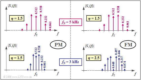
$\text{Example (B)}$ has already been shown that the angle modulation of a harmonic oscillation of the frequency $f_{\rm N}$ leads to a line spectrum. The spectral lines are around the carrier frequency $f_{\rm T}$ bei $f_{\rm T} + n \cdot f_{\rm N}$ with $n \in \{ \ \text{...}, -2, -1, \ 0, +1, +2, \text{...} \ \}$. The weights of the Dirac lines are ${\rm J }_n(\eta)$, depending on the modulation index $\eta$.
The graph shows the magnitude spectrum $\vert S_{\rm +}(f) \vert$ of the analytic signal in phase modulation (PM) and frequency modulation (FM), two different forms of angle modulation (WM). Bessellines with values less than $0.03$ are neglected in both cases.
For the upper half of the image, the modulator parameters are chosen so that for each $f_{\rm N} = 5 \ \rm kHz$ here is a Bessel spectrum with the modulation index $η = 1.5$. Disregarding the phase relationships, the same spectra and the same signals result for both systems.
The lower graphics apply with otherwise identical settings for the same message frequency $f_{\rm N} = 3 \ \rm kHz$. One notices:
- In phase modulation, the spectral function is narrower than $f_{\rm N} = 5 \ \rm kHz$, because the distance of the Bessel lines is now only $3 \ \rm kHz$. Since the modulation index of PM is independent of $f_{\rm N}$, the same bessel weights result as in $f_{\rm N} = 5 \ \rm kHz$.
- Also in the frequency modulation, the Bessel lines now occur at a distance of $3 \ \rm kHz$. However, since FM has a modulation index inversely proportional to $f_{\rm N}$, there are now more significantly more Bessel lines at the bottom due to the larger modulation index $η = 2.5$ than in the upper right (for $η = 1.5$ valid) chart.
Applet Manual
(A) Sum formula of the Bessel functions ${\rm J}_n(x)$
(B) Selection of the order $n$ for the graphical representation
(C) Plot of the Bessel functions
(D) Variation of the graphic representation
$\hspace{1.5cm}$„$+$” (Enlarge),
$\hspace{1.5cm}$ „$-$” (Decrease)
$\hspace{1.5cm}$ „$\rm o$” (Reset to default)
$\hspace{1.5cm}$ „$\leftarrow$” (pushed to the left), usw.
(E) Selection of the abscissa value $x_1$ for the left numeric output
(F) Numerical output of the Bessel function values ${\rm J}_n(x_1)$
(G) Selection of the abscissa value $x_2$ for the right numeric output
(F) Numerical output of the Bessel function values ${\rm J}_n(x_2)$
About the Authors
This interactive applet was designed and realized at the Lehrstuhl für Nachrichtentechnik of the Technische Universität München.
- The original version was created in 2005 by Markus Elsberger and Slim Lamine as part of thesis using „FlashMX–Actionscript” (Supervisor: Günter Söder).
- In 2018 this Applet was redesigned and updated to „HTML5” by Xiaohan Liu as part of her Bachelor's thesis (Supervisor: Tasnád Kernetzky).


